Annotating genomic regions
Learning Objectives
- Annotate GRanges objects with gene features
- Compare and plot annotations of ChIP-seq peaks
- Run functional enrichment analyses on sets of genes
4. Annotating GenomicRanges
As we have seen, there are several different methods to create and import genome annotation data. Bioconductor also has many packages designed to analyse and annotate genomic datasets.
There are several options for annotating GRanges objects with sets of features. Genomation and ChIPpeakAnno for instance all provide methods to do this. There are also packages like Homer and DeepTools available outside of R. Here we are going to use ChIPseeker to annotate sets of ChIP-seq peaks relative to gene annotations.
First, let’s make sure you have the following datasets from previous lessons:
library(TxDb.Hsapiens.UCSC.hg19.knownGene)
library(org.Hs.eg.db)
options(timeout=600) ## This will increase the time for downloading large files

txdb.gff<-makeTxDbFromGFF(file = "http://bifx-core.bio.ed.ac.uk/genomes/human/hg19/annotation/Homo_sapiens.GRCh37.74.edited.gtf",format = "gtf",organism = "Homo sapiens")
4.1 The data
We are going to use data from the ChIPSeeker tutorial which includes ChIP-seq peaks for CBX6 and CBX7 in human fibroblasts, 2 components of the polycomb repressive complex (GEO GSE40740). In addition, there are also ChIP-seq peaks for human andronegen receptor (AR) in cells at 3 different concentrations of andronegen ARmo_0M, ARmo_1nM, ARmo_100nM (GEO GSE48308).
These datasets are all aligned to the human hg19 assembly.
4.2 Annotate peaks
Load the ChIPseeker library and the CBX6 peaks as a GRanges object. The readPeakFile function is provided by ChIPseeker but you could also use readBed from the genomation package.
library(ChIPseeker)
## Get the example file locations
peakFiles <- getSampleFiles()
## Select CBX6 for further analysis
CBX6 <- readPeakFile(peakFiles[[4]])
## Inspect the GRanges object
CBX6
## GRanges object with 1331 ranges and 2 metadata columns:
## seqnames ranges strand | V4 V5
## <Rle> <IRanges> <Rle> | <character> <numeric>
## [1] chr1 815093-817883 * | MACS_peak_1 295.76
## [2] chr1 1243288-1244338 * | MACS_peak_2 63.19
## [3] chr1 2979977-2981228 * | MACS_peak_3 100.16
## [4] chr1 3566182-3567876 * | MACS_peak_4 558.89
## [5] chr1 3816546-3818111 * | MACS_peak_5 57.57
## ... ... ... ... . ... ...
## [1327] chrX 135244783-135245821 * | MACS_peak_1327 55.54
## [1328] chrX 139171964-139173506 * | MACS_peak_1328 270.19
## [1329] chrX 139583954-139586126 * | MACS_peak_1329 918.73
## [1330] chrX 139592002-139593238 * | MACS_peak_1330 210.88
## [1331] chrY 13845134-13845777 * | MACS_peak_1331 58.39
## -------
## seqinfo: 24 sequences from an unspecified genome; no seqlengthsFirst, let’s visualise the distribution of CBX6 peaks along the genome.
## Plot distribution of peaks and peak heights on Chromosomes
covplot(CBX6, weightCol="V5")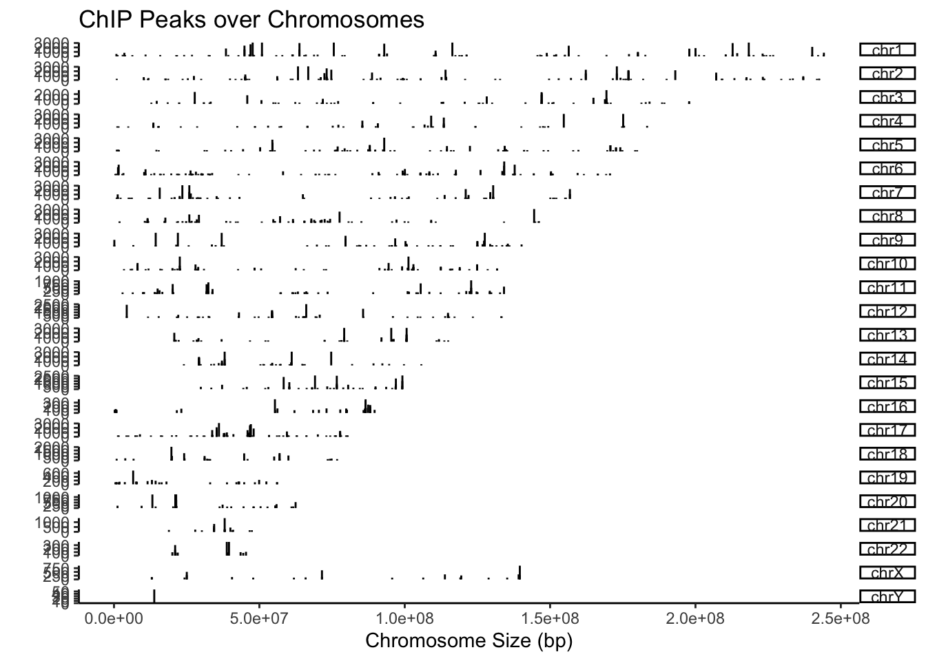
We will now use the txdb object we created earlier to annotate our peaks with gene features. The promoter regions are given as +/- 3Kb around the TSS of each gene.
## Annotate the peak regions with gene features. We can also set the level to "transcript"
peakAnno <- annotatePeak(CBX6, tssRegion=c(-3000, 3000),
                         TxDb=txdb.gff, annoDb="org.Hs.eg.db",level="gene")
## >> preparing features information... 2023-06-05 15:13:49
## >> identifying nearest features... 2023-06-05 15:13:50
## >> calculating distance from peak to TSS... 2023-06-05 15:13:50
## >> assigning genomic annotation... 2023-06-05 15:13:50
## >> adding gene annotation... 2023-06-05 15:14:03
## >> assigning chromosome lengths 2023-06-05 15:14:03
## >> done... 2023-06-05 15:14:03peakAnno## Annotated peaks generated by ChIPseeker
## 1331/1331 peaks were annotated
## Genomic Annotation Summary:
## Feature Frequency
## 9 Promoter (<=1kb) 47.85875282
## 10 Promoter (1-2kb) 7.06235913
## 11 Promoter (2-3kb) 5.10894065
## 4 5' UTR 3.60631104
## 3 3' UTR 2.10368144
## 1 1st Exon 0.52592036
## 7 Other Exon 2.32907588
## 2 1st Intron 5.10894065
## 8 Other Intron 5.48459805
## 6 Downstream (<=300) 0.07513148
## 5 Distal Intergenic 20.73628850This output shows us the distribution of peaks with respect to gene features. The peakAnno object also contains a GRanges object where our peaks are annotated with overlapping features in the metadata.
## Let's look at our annotated GRanges object
as.GRanges(peakAnno)
## GRanges object with 1331 ranges and 13 metadata columns:
## seqnames ranges strand | V4 V5
## <Rle> <IRanges> <Rle> | <character> <numeric>
## [1] chr1 815093-817883 * | MACS_peak_1 295.76
## [2] chr1 1243288-1244338 * | MACS_peak_2 63.19
## [3] chr1 2979977-2981228 * | MACS_peak_3 100.16
## [4] chr1 3566182-3567876 * | MACS_peak_4 558.89
## [5] chr1 3816546-3818111 * | MACS_peak_5 57.57
## ... ... ... ... . ... ...
## [1327] chrX 135244783-135245821 * | MACS_peak_1327 55.54
## [1328] chrX 139171964-139173506 * | MACS_peak_1328 270.19
## [1329] chrX 139583954-139586126 * | MACS_peak_1329 918.73
## [1330] chrX 139592002-139593238 * | MACS_peak_1330 210.88
## [1331] chrY 13845134-13845777 * | MACS_peak_1331 58.39
## annotation geneChr geneStart geneEnd geneLength
## <character> <integer> <integer> <integer> <integer>
## [1] Promoter (<=1kb) 1 818043 819983 1941
## [2] Promoter (<=1kb) 1 1243947 1247057 3111
## [3] Promoter (1-2kb) 1 2978523 2978959 437
## [4] Promoter (1-2kb) 1 3569084 3652765 83682
## [5] Promoter (<=1kb) 1 3805689 3816857 11169
## ... ... ... ... ... ...
## [1327] Intron (ENST00000394.. 23 135229559 135293518 63960
## [1328] Promoter (<=1kb) 23 139173902 139174720 819
## [1329] Promoter (1-2kb) 23 139585152 139587225 2074
## [1330] Distal Intergenic 23 139585152 139587225 2074
## [1331] Distal Intergenic 24 13901758 13903233 1476
## geneStrand geneId distanceToTSS ENTREZID SYMBOL
## <integer> <character> <numeric> <character> <character>
## [1] 1 ENSG00000269308 -160 <NA> <NA>
## [2] 1 ENSG00000169972 0 126789 PUSL1
## [3] 2 ENSG00000256761 -1018 <NA> <NA>
## [4] 1 ENSG00000078900 -1208 7161 TP73
## [5] 2 ENSG00000198912 0 339448 C1orf174
## ... ... ... ... ... ...
## [1327] 1 ENSG00000022267 15224 2273 FHL1
## [1328] 1 ENSG00000230707 -396 389895 LOC389895
## [1329] 2 ENSG00000134595 1099 6658 SOX3
## [1330] 2 ENSG00000134595 -4777 6658 SOX3
## [1331] 2 ENSG00000234385 57456 650983 RCC2P1
## GENENAME
## <character>
## [1] <NA>
## [2] pseudouridine syntha..
## [3] <NA>
## [4] tumor protein p73
## [5] chromosome 1 open re..
## ... ...
## [1327] four and a half LIM ..
## [1328] chromosome 16 open r..
## [1329] SRY-box transcriptio..
## [1330] SRY-box transcriptio..
## [1331] regulator of chromos..
## -------
## seqinfo: 24 sequences from an unspecified genome; no seqlengths4.3 Visualise annotations
We can visualise the distribution of peaks relative to gene features by plotting the peakAnno object.
plotAnnoBar(peakAnno)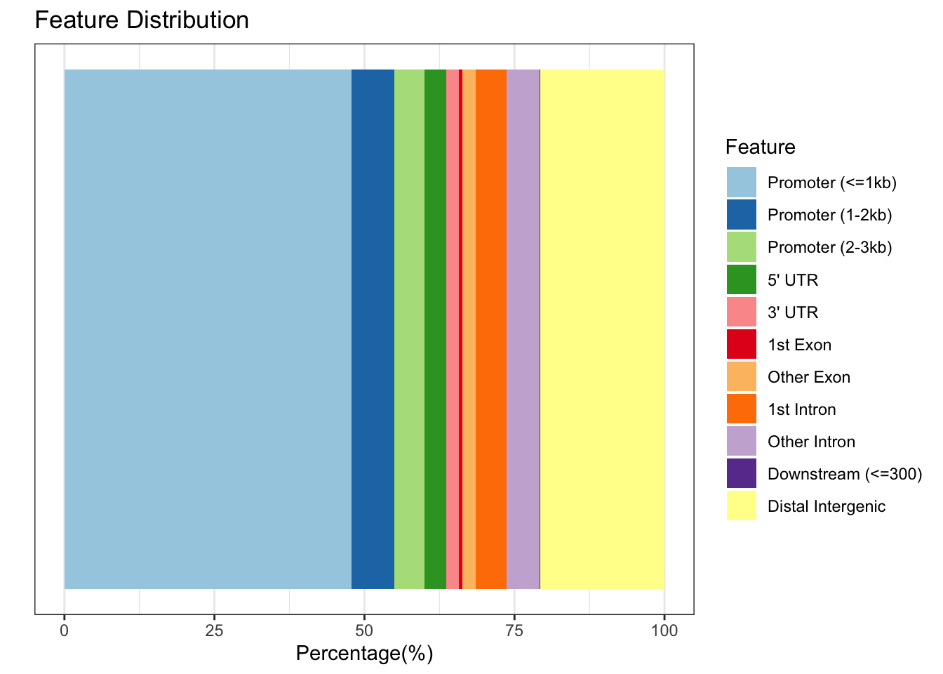
Here we can see that ~60% of our peaks can be found in or around promoter regions.
We can also annotate and plot multiple peaks at once. Let’s use all of the sample datasets within ChIPSeeker. To do this, we use the lapply function in base R to loop through our peak files and run the annotatePeak function.
## lapply loops all of the files through the annotatePeak function to create a list of annotated peaks
peakAnnoList <- lapply(peakFiles, annotatePeak, TxDb=txdb.gff,
                       tssRegion=c(-3000, 3000),annoDb="org.Hs.eg.db",level="gene")
## >> loading peak file... 2023-06-05 15:14:04
## >> preparing features information... 2023-06-05 15:14:04
## >> identifying nearest features... 2023-06-05 15:14:04
## >> calculating distance from peak to TSS... 2023-06-05 15:14:04
## >> assigning genomic annotation... 2023-06-05 15:14:04
## >> adding gene annotation... 2023-06-05 15:14:05
## >> assigning chromosome lengths 2023-06-05 15:14:05
## >> done... 2023-06-05 15:14:05
## >> loading peak file... 2023-06-05 15:14:05
## >> preparing features information... 2023-06-05 15:14:05
## >> identifying nearest features... 2023-06-05 15:14:05
## >> calculating distance from peak to TSS... 2023-06-05 15:14:05
## >> assigning genomic annotation... 2023-06-05 15:14:05
## >> adding gene annotation... 2023-06-05 15:14:07
## >> assigning chromosome lengths 2023-06-05 15:14:07
## >> done... 2023-06-05 15:14:07
## >> loading peak file... 2023-06-05 15:14:07
## >> preparing features information... 2023-06-05 15:14:07
## >> identifying nearest features... 2023-06-05 15:14:07
## >> calculating distance from peak to TSS... 2023-06-05 15:14:07
## >> assigning genomic annotation... 2023-06-05 15:14:07
## >> adding gene annotation... 2023-06-05 15:14:09
## >> assigning chromosome lengths 2023-06-05 15:14:09
## >> done... 2023-06-05 15:14:09
## >> loading peak file... 2023-06-05 15:14:09
## >> preparing features information... 2023-06-05 15:14:09
## >> identifying nearest features... 2023-06-05 15:14:09
## >> calculating distance from peak to TSS... 2023-06-05 15:14:09
## >> assigning genomic annotation... 2023-06-05 15:14:09
## >> adding gene annotation... 2023-06-05 15:14:11
## >> assigning chromosome lengths 2023-06-05 15:14:11
## >> done... 2023-06-05 15:14:11
## >> loading peak file... 2023-06-05 15:14:11
## >> preparing features information... 2023-06-05 15:14:11
## >> identifying nearest features... 2023-06-05 15:14:11
## >> calculating distance from peak to TSS... 2023-06-05 15:14:11
## >> assigning genomic annotation... 2023-06-05 15:14:11
## >> adding gene annotation... 2023-06-05 15:14:13
## >> assigning chromosome lengths 2023-06-05 15:14:13
## >> done... 2023-06-05 15:14:13## Plot all the sets of peaks together
plotAnnoBar(peakAnnoList)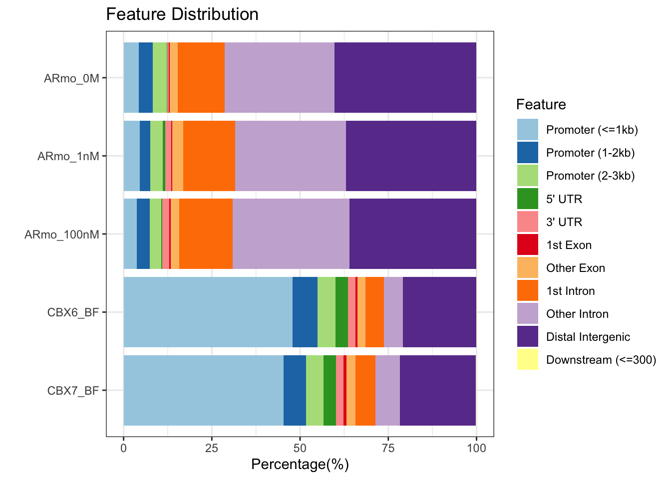
We can clearly see different distributions of peaks in relation to genomic features for the AR and CBX proteins.
4.4 Plot peak distributions around TSS
Let’s plot the positions of peaks for all samples relative to the TSS regions in our gene model. We first need to create a matrix of peaks around the TSS regions. This can take some time so we will use a pre-computed dataset.
## Set the promoter regions
promoter <- getPromoters(TxDb=txdb.gff, upstream=3000, downstream=3000)

## !!! The step below takes around 10 mins to complete, in order to speed up the tutorial the data is supplied below!!!##

## Create a matrix of peak positions for each of the samples. Be patient, this will take around 10 mins to run.
#tagMatrixList <- lapply(peakFiles, getTagMatrix, windows=promoter)
data("tagMatrixList")
We can now plot out the matrix to see the average profile of peaks around promoter regions.
## Plot average profiles of peak distribution across promoter regions
plotAvgProf(tagMatrixList, xlim=c(-3000, 3000), facet="row")
## >> plotting figure... 2023-06-05 15:14:13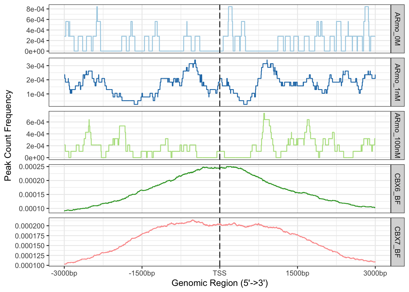
## It is possible to add errors to your plots by adding conf and resample arguments. This will run bootstrapping but will take some time.
#plotAvgProf(tagMatrixList, xlim=c(-3000, 3000), facet="row",conf=0.95,resample=1000)
We can also plot this as a heatmap rather than an average profile.
##Plot heatmaps of peak distribution across promoter regions
tagHeatmap(tagMatrixList,xlim = c(-3000,3000))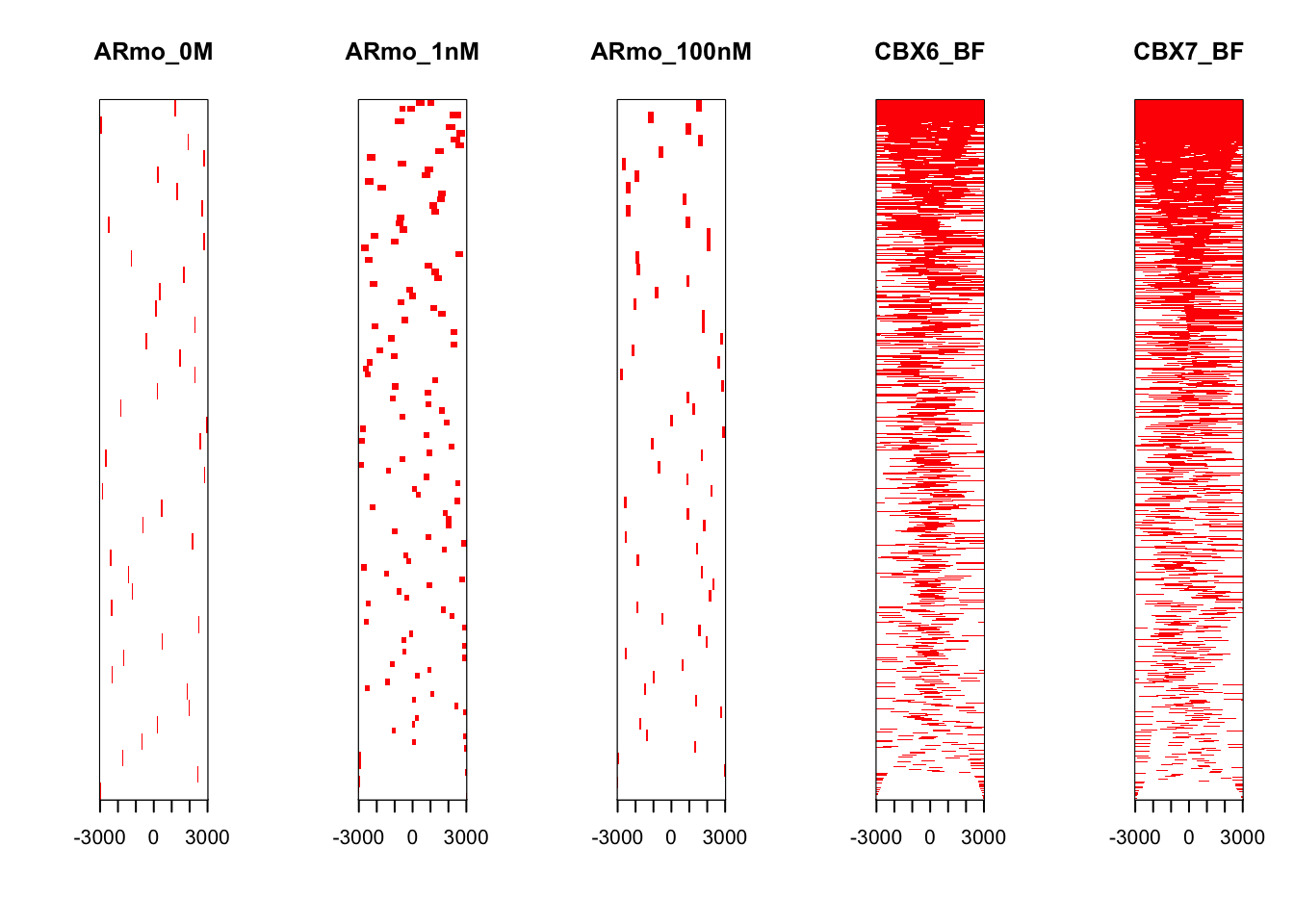
With both plots we can see a definite enrichment of ChIP-seq peaks around the TSS in both CBX6 and CBX7.
Further Learning
If you are working with ChIP-seq data then it is worth going through the ChIP-seeker tutorial as there are many other useful functions:
- Plotting average peak profile across gene bodies and other features
- Functional enrichment analysis
- Venn diagrams of peak set overlaps
4.5 Overlapping features
Genomation and ChIPseeker both have some nice functions for looking at overlaps between GRanges objects:
# Genomation can annotate a GRanges object with another
library(genomation)
par(mfrow=c(1,1)) ## reset plotting format as ChIPseeker has altered this
CBX6.promoters<-annotateWithFeature(CBX6,promoter,feature.name ="Promoters")
CBX6.promoters
## Promoters other
## 60.03 39.97
## [1] 1.64## Plot the annotation overlap as a pie chart
plotTargetAnnotation(CBX6.promoters,col=c("#0B7189","#8FD694"),main="CBX6")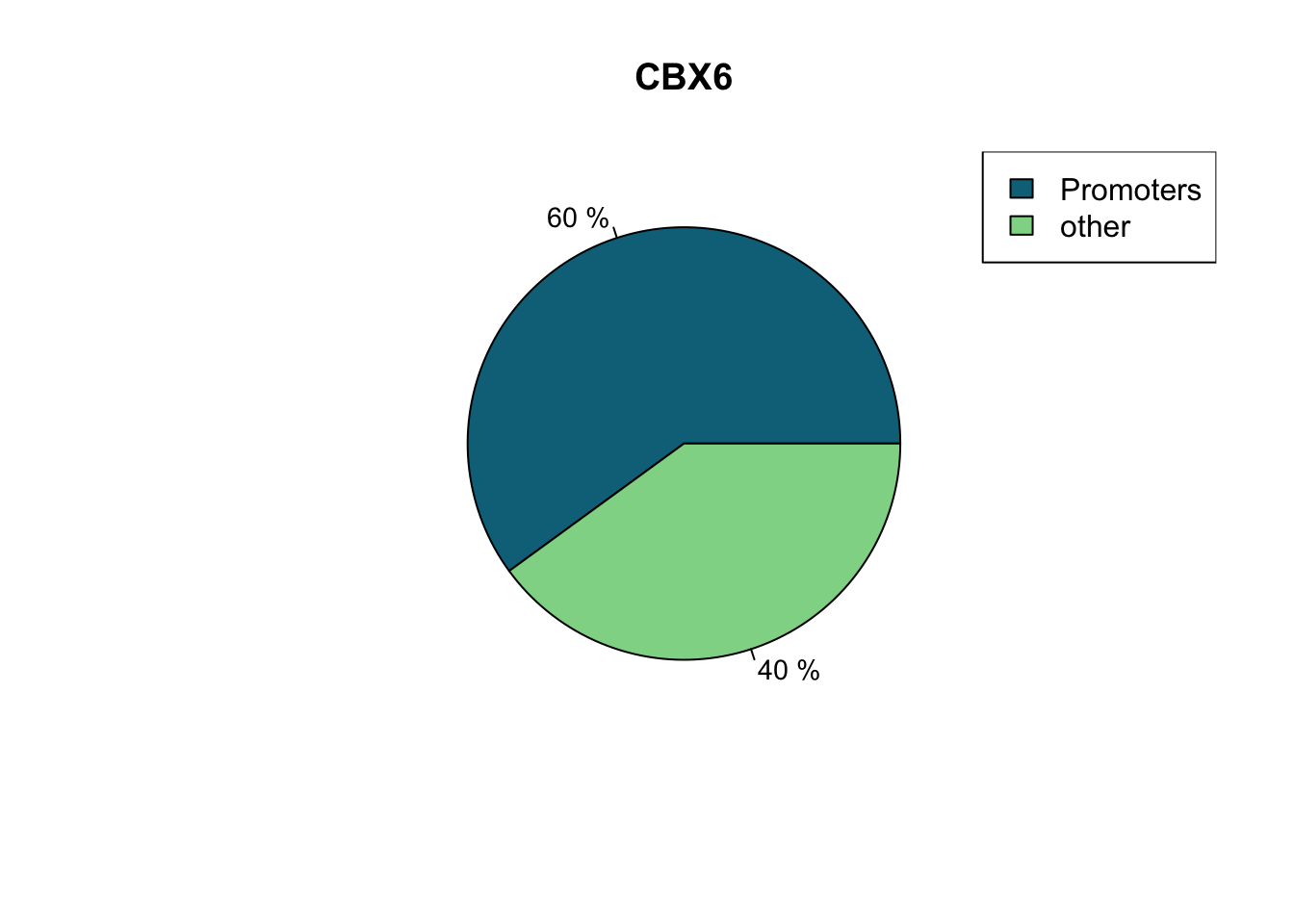
## Read in CBX7 and AR1 files as GRanges
CBX7<-readPeakFile(peakFiles[[5]])
AR1<-readPeakFile(peakFiles[[1]])
## Annotate with multiple features
CBX.overlap<-annotateWithFeatures(CBX6,GRangesList(CBX7=CBX7,AR1=AR1))
CBX.overlap
## CBX7 AR1
## 71.9 0.0
## CBX7 AR1
## 51.17 0.004.6 Statistical testing of overlaps
It is useful to know to what extent peaks from different samples overlap and whether this overlap is statistically significant, as it may imply co-operative binding. ChIPseeker has a function enrichPeakOverlap to calculate and test overlaps between peak sets.
The function generates a null distribution by randomly shuffling the positions of the query peaks throughout the genome and testing for overlaps with the other peaks, then repeating this many times. You should set the nShuffle argument to >=1000 for robust results.
enrichPeakOverlap(queryPeak     = CBX6,
                  targetPeak    = unlist(peakFiles[c(1:3,5)]),
                  TxDb          = txdb.gff,
                  pAdjustMethod = "BH",
                  nShuffle      = 1000,
                  verbose       = FALSE,
                  chainFile     = NULL)
Unfortunately, there seems to be a bug in some versions of ChIPseeker where it will return all p-values as 1. An alternative package, regioneR has a comprehensive set of functions for overlap analysis.
The regioneR package performs association analysis of overlapping features based on permutation tests. The permutation test first calculates the number of overlaps between a genomic feature and a set of given regions. To test if this number is expected by chance it also calculates a distribution of feature overlaps from numerous sets of randomised regions.
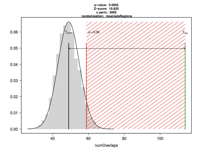
regioneR takes a while to run, so we have supplied the code below as an example but will not run this in the workshop. We can use regioneR to test the significance of overlaps between CBX6 peaks and promoter regions:
library(regioneR)
## Test the significance of overlaps between CBX6 and gene promoter regions.

# pt<-permTest(A=CBX6,B=promoter,randomize.function = randomizeRegions, evaluate.function = numOverlaps,count.once=T,genome="BSgenome.Hsapiens.UCSC.hg19.masked",ntimes=1000)
# pt
# plot(pt)
When using regioneR you need to select an evaluation and randomisation function.
Here we have evaluated the number of overlaps between regions, you can also use the distance between regions or the mean score if your GRanges are weighted (e.g. methylation score).
For randomisation, we have used the randomizeRegions function which selects random regions from the genome with the same length distribution as our CBX6 peaks to approximate the null distribution. We supply a repeat masked BSgenome so only mappable regions of the genome are selected.
The alternative is to use resampleRegions. This assumes that your regions are part of a larger set e.g. differential binding sites. You can then approximate the null distribution by randomly sampling the same number from the full set of binding sites.
Further Learning
All of this is described in depth in the regioneR documentation.
Discussion
Can you think of other situations where we might want to look at overlaps of genomic regions?
- Overlap of ChIP-seq peaks of replicates to test reproducibility
- Overlap of ChIP-seq peaks from different proteins to test for co-localisation
- Overlap of differentially expressed genes with specific genomic
features
- Chromatin marks, classes of repeats, CpG islands etc.
5. Functional gene enrichment
Because we have annotated CBX6 peaks with ChIPseeker we can ask if these genes are enriched for particular functional terms. We can use the clusterProfiler package to perform GO enrichment analysis.
library(clusterProfiler)
## Get the Entrez Gene IDs for genes with a CBX6 binding site.
## na.omit will remove all of the NA entries
CBX6.gene<-na.omit(peakAnno@anno$ENTREZID)

##Run the GO enrichment analysis
ego <- enrichGO(gene          = CBX6.gene,
                OrgDb         = org.Hs.eg.db,
                ont           = "ALL",
                pAdjustMethod = "BH",
                pvalueCutoff  = 0.01,
                qvalueCutoff  = 0.05,
                readable      = TRUE)
head(ego)
##Plot the top enriched terms
barplot(ego, showCategory=20,colorBy = "p.adjust")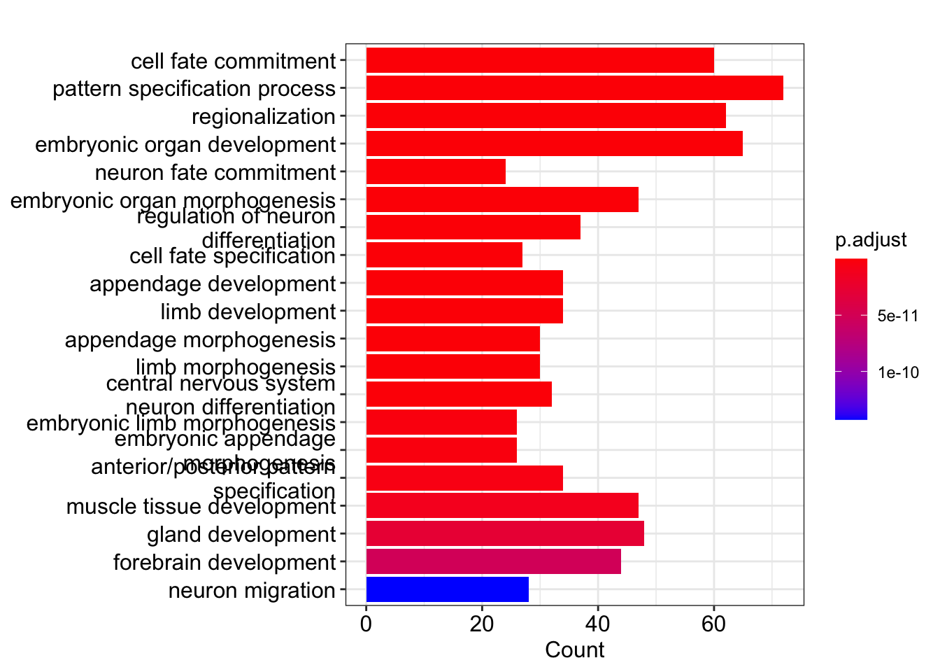
Further Learning
clusterProfiler also provides methods to query pathway databases such as KEGG. You can find out more in the documentation.
The package gprofiler2 is a wrapper for the online tool g:Profiler and looks at many different databases at once including GO, KEGG and transcription factor motifs. g:Profiler performs functional enrichment analysis of gene lists and will understand and convert Ensembl identifiers directly.
library(gprofiler2)
##Get a table of enriched terms with the gost function
gp<-gost(query = peakAnno@anno$geneId,organism = "hsapiens", ordered_query = FALSE,
                multi_query = FALSE, significant = TRUE, exclude_iea = TRUE,
                user_threshold = 0.05, correction_method = "g_SCS",
                domain_scope = "annotated", custom_bg = NULL)

##Inspect the output, the "term_name" column is the enriched term and the "source" tells us which database it belongs to.
gp$result
There is an interactive plot function built into gprofiler2 to visualise enriched terms.
## Plot gprofiler output
gostplot(gp, capped = TRUE, interactive = TRUE)
Challenge:
See if you can produce a list of GO terms that are enriched in both the clusterProfiler and gprofiler2 outputs.Solution:
ego[ego$ID %in% gp$result$term_id,1:3]Key points
- You can annotate GRanges objects with packages like genomation and ChIPseeker