Getting Started
We recommend using RStudio for this workshop. RStudio is an Integrated Development Environment (IDE) for R. It can be accessed in several ways. Download RStudio and install it on your own computer.
Using RStudio
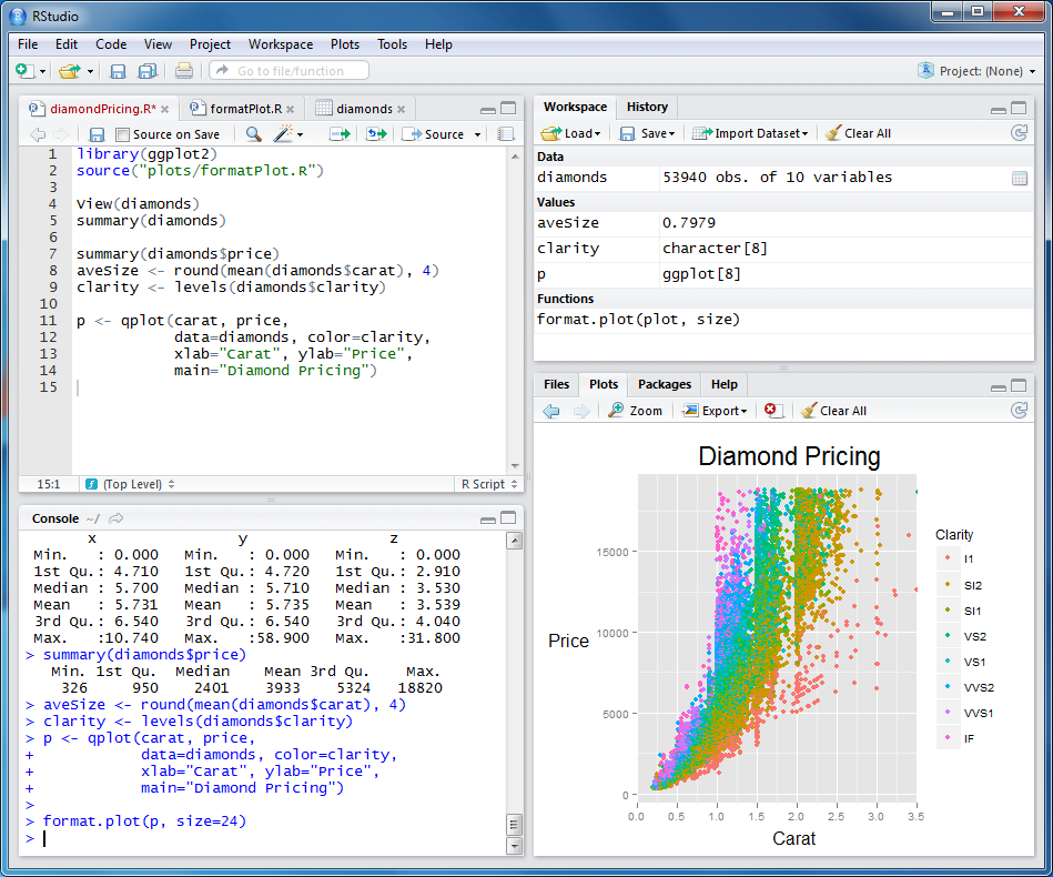
The are 4 main panes, each with several tabs:
- Console (bottom left)
- Here you can type commands into R
- Additional tabs may include a terminal and script outputs
- Editor (top left)
- Open and view files
- These can be raw txt, scripts or markdown
- Environment (top right)
- Objects you have stored
- Commands you have typed
- Additional tabs for version control, database and website building…
- Files and output (bottom right)
- System files (on the computer/server you are working on)
- Output from plots or applications
- Packages available
- Help pages

You can cutomise the appearance of RStudio under the Tools -> Global Options… menu.
Setting up a new project
There is a drop-down project menu at the top right of RStudio. Click this, select “New Project…” and create one in a new directory. Make sure you have write permission for the directory you choose.
Once you have done this, this will be your working directory. Files will be saved (or loaded from) here by default unless you specify a full path. You can change your working directory under the session menu at the top.
Using Rstudio has the advantage that everything you do can be saved between RStudio sessions.
Running commands
You can work in 3 different ways in RStudio.
- Use the console to run commands.
- Create a new R script to save your commands as you go.
- Create an R markdown file to generate web pages or pdf documents from your analyses.
Commands can be typed directly into the console, but in order to keep track it’s best to write them into a script as you go (File->New File->R Script). From here you can use a shortcut to run the command on the line where your cursor is:
- Alt + Enter to keep the cursor on the same line
- Ctrl + Enter to move to the next line
You can also use the Tab key to autocomplete names of functions and objects as you type them into your script.
Hint: When using the console, the Up/Down arrow keys can be use to cycle through previous commands.
In the console you should always see a > prompt, if
you can’t see this R may still be working. There is a red Stop light at
the top right of the console when a command is running. If you see a
+ instead of >, R is waiting for more
input. Sometimes this means you have forgotten to close a bracket or
quotation.
Using R Markdown is a great way to annotate your code and present an analysis with code, figures and text all together in a web page or document format. It’s worth learning but adds a further level of complication for novice users so is not covered in this course.
Installing libraries
Libraries provide additional functions in R and can be downloaded from several sources:
- CRAN is the Comprehensive R Archive Network and hosts the majority of generic R packages.
- Bioconductor is a repository of biology specific packages.
- Third party tools are often hosted on github.
Install the packages we need for these lessons by running the code below in the R console:
#install from CRAN with install.packages()
install.packages(c("tidyverse", "ggthemes", "plotly","ggpubr", "ggrepel","viridis","RColorBrewer","ggsci","patchwork","gghighlight","rstatix"))

#Example to install from bioconductor with BiocManager
#if (!requireNamespace("BiocManager", quietly = TRUE))
#    install.packages("BiocManager")
#BiocManager::install(c("DESeq2","genomation"))

#Example to install from github with the devtools package
#install.packages("devtools")
#devtools::install_github("thomasp85/patchwork")
To load a specific package within an R session, use the
library function:
library(tidyverse)How to follow this tutorial
- Create a new project in RStudio
- Install the required libraries
- Open a new R script (or R markdown file for advanced users)
- It will be best to work with the tutorial and RStudio open together so you can easily switch between the two. Working on a wide split-screen or multiple desktops is the best setup.
- I recommend typing out commands rather than copy-and-pasting if you want to learn. Remember you can use the Tab key to save yourself from endless typing!